AI System Introduction

AI Infrastructure stack can be broadly categorized in 4 major layers: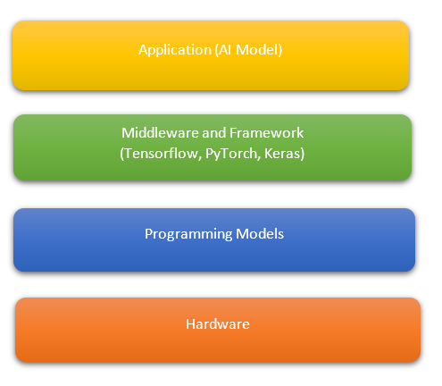

• The first layer is called the application layer where we execute our AI application software.
• The second layer is called the middleware and framework layer which comprise AI and ML frameworks e.g. Tensorflow, PyTorch, Keras, etc.
• The third layer is called the programming model layer and is the lowest layer of the software that is closest to the hardware and interacts with the layer above to create optimized code for the specific architecture being targeted, e.g. x86, ARM, etc. This layer is majorly written by library developers having expertise in hardware/ software interaction. This is the layer where AI specific hardware features and interactions are leveraged to accelerate AI software.
• The fourth layer is the hardware layer which comprise either CPU, GPU, AI accelerators for execution of AI software code.

Artificial Intelligence and Machine Learning rapid uptake over recent years can be attributed not only to new software platforms helping to orchestrate AI and recent advancements in AI models, but also to advancements in the core hardware enabling information processing across massive volumes of data. This has lead to more attraction and new possibilities to build and deploy AI applications in a streamlined fashion. With the rise of GPU (general-purpose parallel processing) as well as AI-focused ASICs (application-specific processing), like TPUs (Tensor Processing Units), engineers today are able to analyze large amount of data in a cost-effective and scalable manner and answer high-impact operational questions.

Based on the user requirement e.g. online/ realtime response for inference for language translation, online prediction vs offline batch inference prediction, the workload can be optimized to take advantage of the unique aspects of different architectures. The model parameters are increasing exponentially, some of the models today have more than 300 trillion parameters. In order to execute these models, hardware clusters are created and the execution jobs are distributed amongst these clusters. The splitting is one of the key areas where innovation continues to find the best way to distribute workloads across devices.

Model Optimization techniques

With such huge models come the huge computational cost for inference and training these models in cloud infrastructure. AI model optimization becomes a key aspect to reduce the cost and can be performed in both training and inference. Following are the few optimization techniques:

• Quantization : quantization is where we reduce the number of bits used to represent our data and weights, e.g. reducing 32 bit number to 16 bit and 8 bit number. This reduction with bits when combined with an architecture can result in significant increase in performance or to reduction in power or both. Challenge is how to map these values from higher number of bits to lower number of bits and maintain an acceptable performance.
• Pruning is another optimization of deep learning models that reduces the size of the model by finding small weights and setting them to zero. Deep learning models typically have large number of weights very close to zero which have minimal contribution to model inference, hence can be ignored. There are several approached to prune a model:
  • Structured and Unstructured techniques: In unstructured technique we remove the weights on a case to case basis whereas in structured approach we remove weights in groups e.g- removing entire channel at a time. Structured pruning typically has better run-time performance characteristics but also has a heavier impact on accuracy of the model
  • Scoring : This approach takes into consideration the threshold value to discard weights . this threshold value is either computed using L1 pruning scores by computing their contribution to the overall tensor vector using taxicab distance or using L2 pruning score computing using Euclidean distance.
  • Scheduling : : In this approach we add additional steps in the training process to prune the model after few epochs. This is also applied in between fine-tuning steps.
• Knowledge Distillation: Knowledge distillation is another technique of model optimization in which we transfer the knowledge from a large to a smaller model that can be practically deployed under real-world constraints. A small student model learns to mimic a large teacher model and leverage the knowledge of the teacher to obtain similar accuracy.

OneDNN, CuDNN are some of the libraries that are highly optimized for linear algebra operations that executes fast on the targeted hardware backend.

AI/ML Model Instruction Analysis

If we closely analyse the Neural networks operations majority of them are general matrix multiplication computations. These can be decomposed into several multiply and addition or MAC operations which can execute in parallel. Hence, hardware supporting high number of MAC operations execution in parallel (e.g. GPU) can be advantageous in training process.

During backpropagation stage each training iteration, we need to use the output from each layer that were computed in the forward propagation stage. These values are typically stored in memory after being computed during the forward propagation and read back and used during back propagation. Thus, a training iteration involves moving large amount of data from compute to memory and vice versa. Therefore, hardware supporting high bandwidth between to compute units and memory can be advantageous in the training process, infact bandwidth is a critical bottleneck across several training workloads.

Low latency is more critical to real world inference applications. Unlike in training, during inference it is more common to process just or very few samples at a time, rather than a large batch of samples to meet the latency requirements of the application. This means for Inference the matrix vector multiplication are more common than GEMMs. Matrix vector multiplication still benefits from parallelism but have less parallelism than general matrix multiplications. Deep Learning applications used to be primarily around image classification nd other visual tasks. Vision remains largest workload in edge applications such as security camera, autonomous vehicles. Recommendation and language tasks dominate across the companies with the largest global data centers. Neural Networks for language and recommendation system are not only growing in number of weights but also in their complexity.

Trends in new Neural Network models

Traditional neural network models comprises sequential layers and the inputs and outputs are of static sizes. Newer neural networks have dynamic inputs and outputs sizes and are adopting a cross structure where the outputs of several non-sequential layer can become input to another layer. The computational pattern and memory accesses are predictable for traditional neural networks as they required a lot of MACs i.e. Multiply and Addition operations and therefore required high memory bandwidth for training. The predictable nature of computation patterns made it simpler for the software to pipeline the data to efficiently use the hardware.

Newer Neural networks have more irregular memory access patterns and in addition to MACs and bandwidth they also require larger memory capacity, high operating frequency for the growing number of non parallelize computations and lower memory read and write latencies across non-sequential memory addresses. Memory and bandwidth are becoming the central components in deep learning system designs. Hardware managed memory or caches consume more power whereas software managed memory or scratchpads typically used in dedicated AI processors or ASICs increase the software complexity.

The continued exponential growth in MACs for silicon area, the memory bandwidth and the bandwidth nodes within a server and across servers are becoming the limiting factors to improve performance. One way to reduce memory and bandwidth consumption is to use less bits to represent numbers, lower numerical precision reduces the memory and bandwidth bottlenecks. On the other hand it can result in lower accuracy, hence one needs to consider the trade-offs from the computational gains with possible accuracy impact.