AI Inference: Models, Systems, and Optimization
Published:
AI Inference: Models, Systems, and Optimization
Inference is the systems problem of turning a trained model into a useful service: one that is responsive, reliable, and affordable under real traffic. For large language models (LLMs), that means coordinating model architecture, GPU memory, kernels, batching, networking, and request scheduling—not merely executing a forward pass.
This post develops a practical mental model for that stack. The central theme is simple: the best optimization depends on the bottleneck, and the bottleneck changes as the model, context length, batch size, and hardware configuration change.
1. Introduction: Why inference has become the new bottleneck
Training receives attention because it is visibly expensive, but inference is where a model’s cost is paid repeatedly. A production model may serve millions of requests, generate billions of tokens, maintain long contexts, call tools, and route requests across GPU clusters. The cumulative serving cost can dominate the cost of a one-time training run.
Training and inference optimize different objectives:
| Training | Inference |
|---|---|
| Maximize samples or tokens per second | Balance latency, throughput, memory, cost, quality, and availability |
| Backward pass plus optimizer state | Forward pass plus persistent KV cache |
| Large, regular batches | Variable-length, latency-sensitive requests |
| Parameters change every step | Parameters are fixed, but execution plans change per request |
For an interactive assistant, time to first token matters. For a batch API, total throughput and dollars per million tokens may matter more. For a reasoning agent, the right trade-off may be to spend more inference compute on hard tasks. There is no universal definition of “fast inference”; performance is always workload-specific.
2. What actually happens during LLM inference
At a high level, an LLM maps a sequence of token IDs to a probability distribution over the next token, samples or selects a token, appends it to the sequence, and repeats.
prompt → tokenize → embeddings → transformer layers → logits → sample next token
                                                        ↑                 │
                                                        └─────────────────┘
Tokenization
Text is first converted into tokens—integer IDs from a model-specific vocabulary. Tokens are not necessarily words: common strings may be single tokens, while rare strings may be split into several pieces. Tokenization affects serving directly because prompt length, output length, cache usage, and billing are usually measured in tokens.
"Explain how GPUs work." → [token_1, token_2, token_3, token_4, token_5]
The IDs index an embedding table. Positional information is added or applied so the transformer can distinguish token order.
Transformer execution
Each transformer layer typically contains attention, a feed-forward network (FFN), normalization, and residual connections:
x → normalization → attention ─┐
│                               ├→ residual → normalization → FFN ─┐
└───────────────────────────────┘                                  ├→ residual
                                                                    └────────────
Self-attention is commonly written as:
$ \operatorname{Attention}(Q,K,V)=\operatorname{softmax}\left(\frac{QK^T}{\sqrt{d}}\right)V $
where $ (Q) $, $ (K) $ , and $ (V) $ are query, key, and value tensors and $ (d) $ is the head dimension. FFNs contain much of the parameter count and are generally implemented as matrix multiplications plus elementwise operations. The output of the final layer is projected into vocabulary logits, then a decoding policy (greedy, temperature sampling, top-p, and so on) chooses the next token.
Prefill
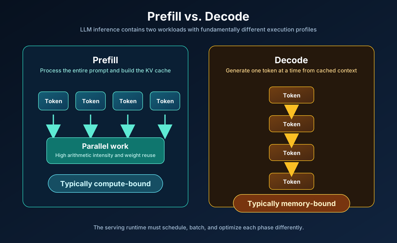
Prefill processes the input prompt and creates the initial KV cache. A 4,000-token prompt has substantial parallel work: many token positions can be evaluated together, subject to causal masking. Its primary user-visible metric is time to first token (TTFT).
prompt tokens ──parallel transformer execution──→ first output token + KV cache
Prefill often has high arithmetic intensity and can be compute-bound, especially for sufficiently long prompts or large batches. Long prompts can still be expensive because attention and cache writes scale with sequence length.
Decode
Decode generates output autoregressively. Each new token depends on the preceding sequence, so a single request exposes little token-level parallelism:
token 1 → token 2 → token 3 → ... → token N
Decode is commonly measured by time per output token (TPOT) or inter-token latency (ITL). With small batches, it is frequently limited by reading model weights and cached states from high-bandwidth memory (HBM), rather than by peak floating-point capability.
3. Why inference is difficult
Model weights
The first constraint is capacity. At FP16/BF16, a dense model requires roughly two bytes per parameter before runtime overhead:
$ M_{weights}\approx 2P\ \text{bytes} $
Thus a 70B-parameter dense model needs about 140 GB just for weights. This does not include the KV cache, temporary activations, communication buffers, or runtime workspace. Whether the weights fit determines the minimum number of GPUs and the parallelism strategy.
Memory bandwidth
During decode, a GPU may repeatedly stream large weight matrices from HBM for only a small amount of work per request. If the batch is too small to reuse those weights effectively, the GPU waits for memory. A useful first-order metric is arithmetic intensity:
$ \text{Arithmetic intensity}=\frac{\text{operations}}{\text{bytes moved}} $
Low arithmetic intensity tends to be memory-bound; high arithmetic intensity can be compute-bound. The roofline model formalizes this: attainable performance is limited by the lower of peak compute and memory-bandwidth times arithmetic intensity.
KV cache
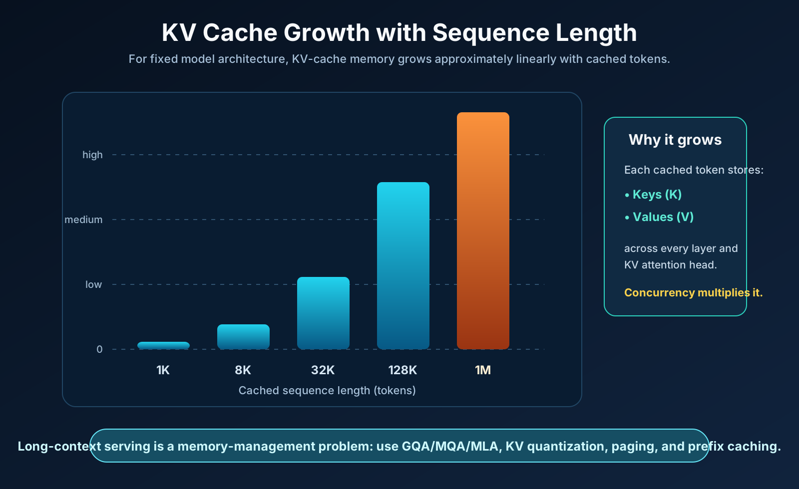
The KV cache stores prior keys and values so the model does not recompute them for every decode step. It removes enormous redundant computation, but it consumes memory proportional to active sequence length and concurrency.
For a simplified attention implementation:
$ M_{KV}\approx 2\times L\times T\times H_{KV}\times D\times B $
where $ (L) $ is layers, $ (T) $ cached tokens, $ (H_{KV}) $ KV heads, $ (D) $ head dimension, and $ (B) $ bytes per element. The factor of two represents keys and values. Real implementations also have alignment and block-management overhead.
Long context turns cache management into a first-class systems problem. A service must decide which sequences may coexist, where their blocks reside, when prefixes can be reused, and whether parts of the cache can be quantized or offloaded.
Compute-bound versus memory-bound phases
Prefill and decode are not merely different points on one curve. They often have different bottlenecks:
| Property | Prefill | Decode |
|---|---|---|
| Parallelism | High across prompt positions | Limited by autoregression |
| Main metric | TTFT | TPOT / ITL |
| Common bottleneck | Compute | HBM bandwidth, KV reads |
| Scheduling goal | Admit and process prompts quickly | Keep an efficient active batch |
This distinction is why a system can have excellent TTFT yet feel slow while streaming, or vice versa.
Latency versus throughput
Batching increases weight reuse and throughput, but queues requests and can worsen tail latency. The scheduler must balance:
larger batch → higher utilization and throughput
larger batch → more queueing, more cache use, potentially worse TTFT/ITL
Production targets should include both central and tail metrics: P50/P95/P99 TTFT, P50/P95 TPOT, tokens per second, request rate, cache hit rate, and cost per token.
Multi-GPU communication
Once a model spans devices, every parallelism scheme creates collective communication. Tensor parallelism requires synchronization of partial results; pipeline parallelism sends activations between stages; expert parallelism performs token routing and all-to-all exchanges. A workload that looks compute-efficient on one GPU can become network-bound on many GPUs.
4. The anatomy of an inference system
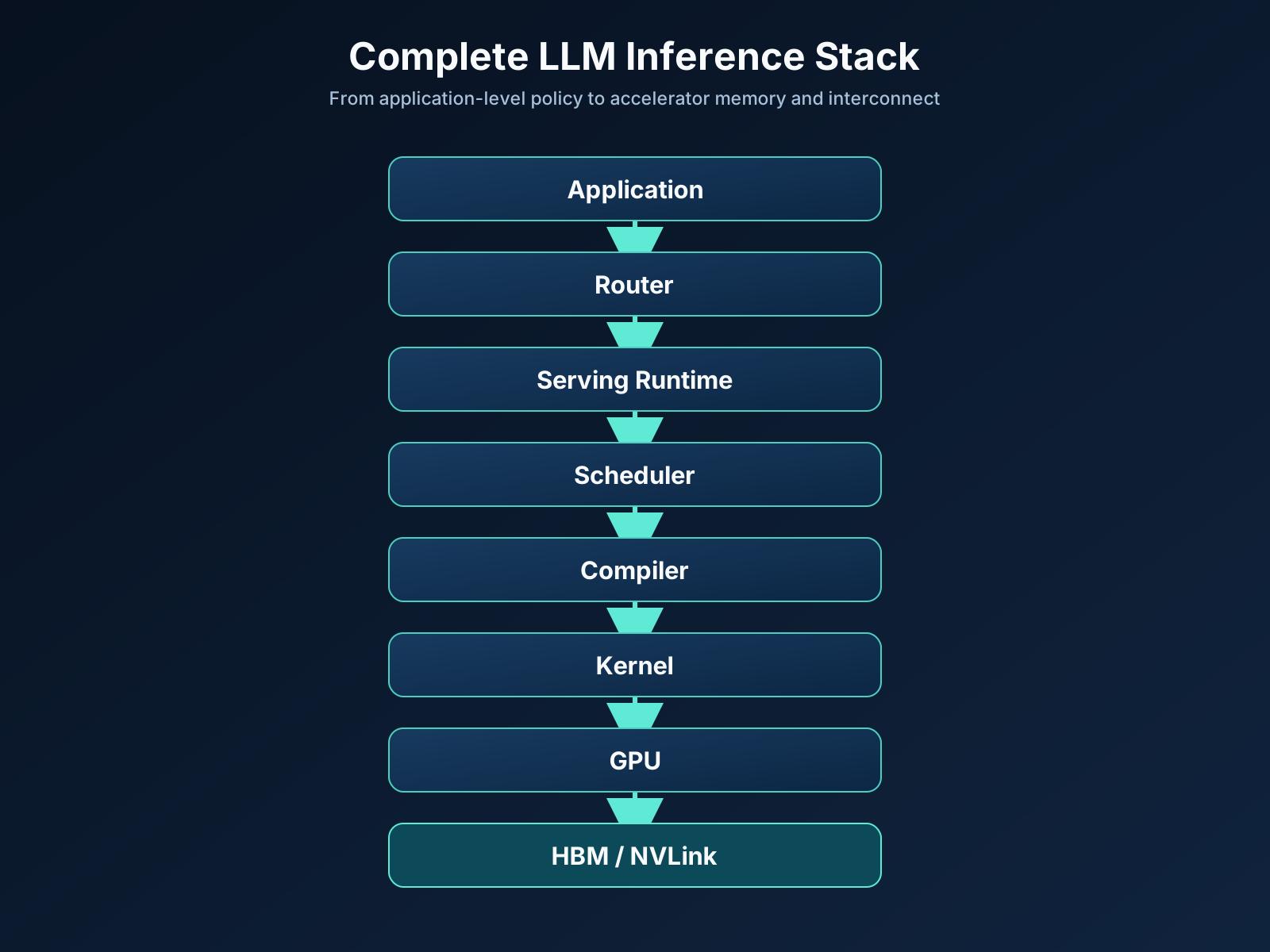
An inference service is a cross-layer stack:
request → router/scheduler → runtime → compiled graph and kernels → GPUs → interconnect
                         ↘ KV-cache manager ↗
Model
The model defines the fundamental work: layer count, hidden size, attention type, vocabulary, precision tolerance, context window, and whether execution is dense or sparse. Architecture choices such as grouped-query attention (GQA), multi-query attention (MQA), multi-head latent attention (MLA), and mixture of experts (MoE) are serving decisions as much as modeling decisions.
Compiler
The compiler lowers model operations into an executable graph. It can specialize shapes, choose tensor layouts, fuse operations, plan memory, select kernels, and capture stable execution paths. Compiler specialization improves efficiency, but highly dynamic request shapes can reduce how often an ideal static plan applies.
Runtime
The runtime owns tensors, streams, memory pools, collective communication, model replicas, and the KV cache. It executes the compiled graph repeatedly, handles admission control, and exposes the service interface. In practice, the runtime is where model-level capabilities become a serving system.
Scheduler
The scheduler decides which requests prefill, which sequences decode next, how much work fits in the active batch, and when to evict or reuse cache blocks. Continuous batching makes this a per-step decision rather than a one-time static batch:
step 1: A B C
step 2: A B C D       (D admitted)
step 3:   B D E       (A/C finished; E admitted)
Kernels
Kernels implement the hot operations: GEMMs, attention, normalization, activations, sampling, and communication. Their performance depends on tiling, tensor-core usage, memory coalescing, occupancy, register pressure, shared memory, and synchronization. A small kernel inefficiency can matter greatly because it repeats across every layer and token.
GPU
Relevant GPU properties are not just FLOPS: HBM capacity, HBM bandwidth, tensor-core performance at the chosen precision, cache hierarchy, and support for low-precision formats all affect serving. A device with more peak compute is not automatically faster for memory-bound decode.
Network
NVLink/NVSwitch-class local interconnects and cluster networking determine the cost of collectives and MoE routing. Topology matters: an all-to-all pattern over a slow or oversubscribed fabric can dominate token latency even when individual GPUs are underutilized.
5. Inference optimization techniques
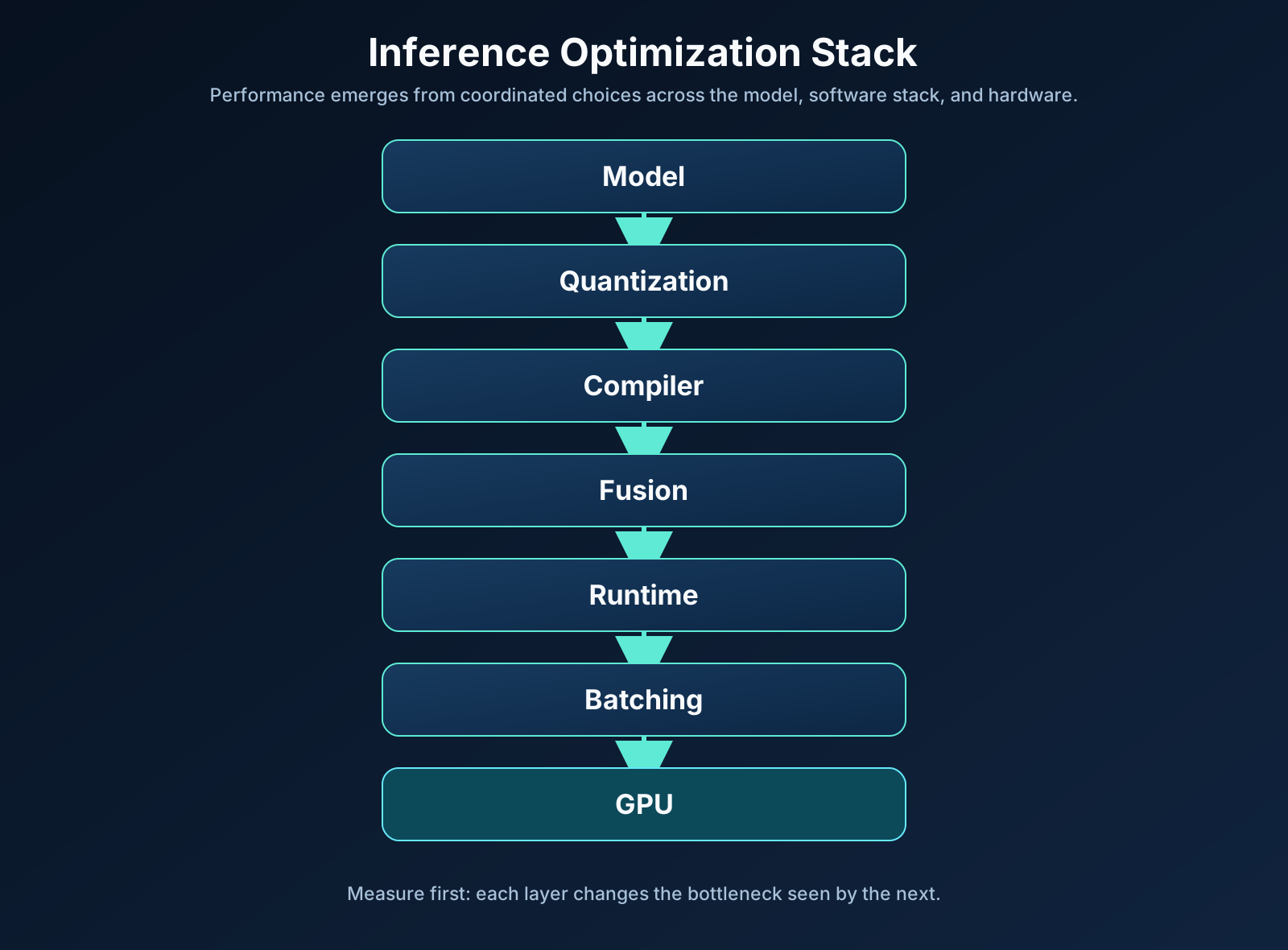
The techniques below attack different resources. They are complementary, not a checklist to apply blindly.
Quantization
Quantization stores and/or computes tensors in lower precision: FP16/BF16, FP8, INT8, INT4, and increasingly FP4-class formats depending on hardware and model support. Weight-only quantization primarily reduces capacity and weight-read bandwidth; activation and KV quantization can further reduce traffic and memory.
The trade-off is numerical error and sometimes dequantization overhead. Validate quality on the workload that matters, including long-context and tool-use cases—not only a generic benchmark.
Kernel fusion
Fusion combines adjacent operations, such as bias addition, activation, normalization, or residual updates, into fewer kernels. It reduces launch overhead and avoids writing intermediate tensors to HBM. Fusion can be especially valuable for decode, where small repeated operations accumulate.
FlashAttention
FlashAttention-style kernels compute attention in tiles and avoid materializing the full attention-score matrix in HBM. The key benefit is lower memory traffic through carefully managed on-chip memory and numerically stable online softmax. It improves attention efficiency, especially as sequence length grows, but does not remove the linear growth of stored KV states.
GQA, MQA, and MLA
Standard multi-head attention has separate K/V states per query head. MQA shares K/V across query heads; GQA shares them within groups. Both reduce KV-cache size and bandwidth at some architectural trade-off.
MLA takes a different route: it stores a compressed latent representation from which attention states are reconstructed or used efficiently. Its serving importance is the same: reduce persistent per-token memory so longer contexts and higher concurrency fit.
KV-cache optimization
KV optimization includes lower-precision storage, layout tuning, block allocation, eviction policies, tiered memory, and cache-aware admission control. The right policy depends on the workload: a long-context agent, a short chat session, and a shared-document assistant have very different reuse patterns.
Continuous batching
Instead of waiting for fixed batches to finish together, continuous batching admits, removes, and schedules sequences at decode-step granularity. It minimizes padding and keeps devices busy despite different output lengths. The scheduler must still protect TTFT and tail ITL from excessive queueing.
Paged KV cache
Paged attention stores each sequence’s cache in fixed-size blocks rather than one contiguous allocation. This limits fragmentation, permits noncontiguous logical sequences, and makes blocks easier to allocate, reclaim, and share. It is analogous to virtual memory: logical token positions map to physical cache blocks.
Prefix caching
When requests share a prefix—such as a system prompt, document, or tool schema—the prefill KV state for that prefix can be reused. Prefix caching can reduce TTFT and compute dramatically, but cache keys must include every model-relevant input and invalidation needs careful design.
Speculative decoding
A fast draft model proposes several tokens; the target model verifies them in fewer target-model iterations than normal autoregressive decoding. The benefit depends on acceptance rate and the extra cost of drafting and verification. It is most useful when the draft is cheap and predicts the target well.
MoE
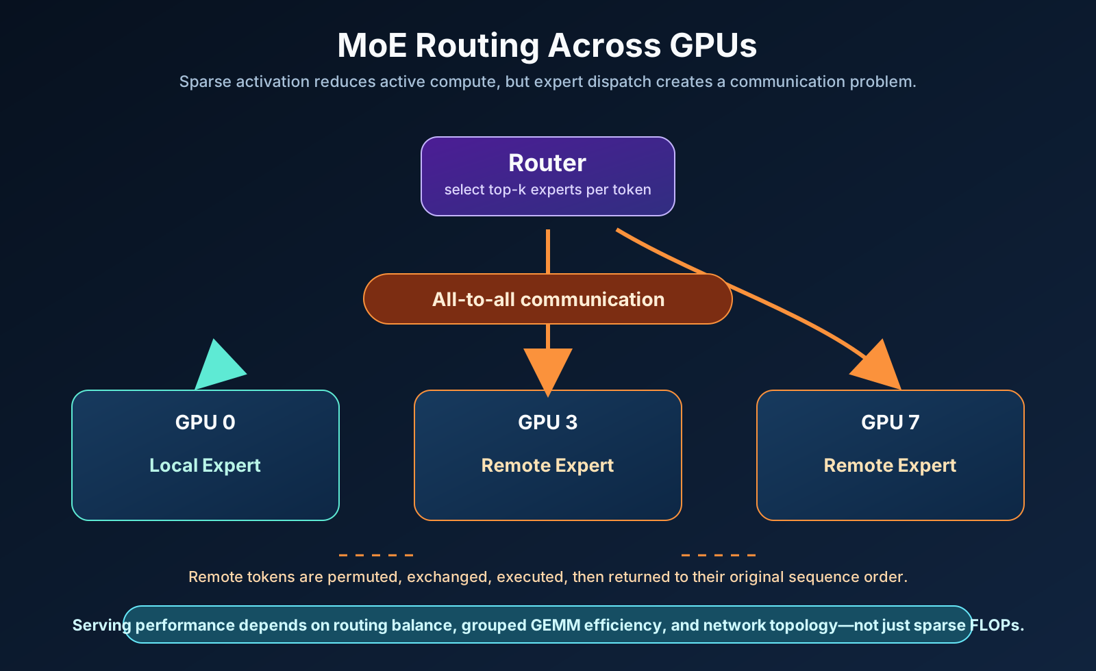
MoE models route each token to a small subset of FFN experts. They decouple total parameter capacity from active parameters per token:
large expert pool → router selects top-k experts → only selected experts execute
MoE reduces active compute but introduces routing, grouped-GEMM, load-balancing, and all-to-all communication challenges. Sparse FLOPs do not guarantee low latency if communication is inefficient.
Parallelism
Tensor parallelism shards individual matrix operations across GPUs. Pipeline parallelism assigns layers to stages. Data parallelism replicates the model across independent request streams. Expert parallelism places MoE experts on different devices. Real deployments commonly use a hybrid, chosen from memory capacity, batch size, topology, and latency targets.
Prefill/decode disaggregation
Because prefill and decode have different shapes and bottlenecks, they can be served by different pools. A prefill pool can optimize prompt processing and TTFT; a decode pool can optimize sustained token generation and cache residency. The difficult part is efficiently transferring KV state and maintaining scheduling stability across pools.
Compiler optimization
Ahead-of-time or just-in-time compilation can fuse operators, select shape-specific kernels, optimize layouts, plan workspace, and overlap communication with computation. Measure compile-time specialization against workload variability: a highly optimized plan for one shape is not automatically ideal for every request.
6. Worked example: optimizing a 70B / 400B model
This example is illustrative rather than a hardware sizing prescription. Exact results depend on architecture, context length, precision, GPU generation, interconnect, and target SLOs.
FP16 baseline
A dense 70B model at FP16 needs roughly 140 GB of weights; a dense 400B model needs roughly 800 GB.
| Model | FP16 weights only | Immediate implication |
|---|---|---|
| 70B dense | ~140 GB | Does not fit on one 80 GB GPU |
| 400B dense | ~800 GB | Requires many devices before cache/workspace |
The baseline should measure TTFT, TPOT, tokens/s, GPU memory, HBM utilization, active batch size, and P95/P99 latency. Without this profile, optimization is guesswork.
Quantization
Moving weights from FP16 to 8-bit roughly halves weight storage; 4-bit weight formats reduce it further, subject to scale/metadata overhead. For a 70B model, the engineering question becomes whether the quantized kernels preserve quality and actually improve decode throughput on the target GPU. For a 400B model, quantization may also reduce the number of shards and collectives required.
GPU memory budget
Do not size hardware from weights alone:
GPU memory = weights + KV cache + activations + workspace + communication buffers + allocator headroom
Increasing concurrency or context length grows the KV portion. A configuration that fits the model may still fail its latency SLO because the usable cache budget is too small.
Tensor parallelism
Shard a 70B model across enough GPUs to meet the capacity budget, then examine collectives on every layer. More tensor-parallel ranks reduce per-GPU weight capacity but increase communication frequency. The optimal point is not necessarily the maximum number of GPUs.
For a 400B dense model, tensor parallelism alone may be insufficient or communication-heavy; a hybrid tensor/pipeline configuration may be appropriate. The topology should keep high-frequency traffic inside the fastest interconnect domain whenever possible.
KV cache
Calculate cache requirements using the model’s actual layer count, KV-head count, head dimension, cache precision, context policy, and concurrent sequences. Then test a paging strategy and, if supported, KV quantization. If cache pressure causes frequent eviction or admission stalls, weight quantization alone will not solve the workload.
Batching
Enable continuous batching, then tune the admission policy against TTFT and TPOT targets. Large batches can convert a memory-bound decode into a more compute-efficient workload through weight reuse, but at the cost of queueing and cache pressure. Separate short and long requests if one class harms the other’s tails.
Identify changing bottlenecks
Optimization is a loop, not a linear recipe:
FP16 baseline: capacity / HBM bandwidth bound
        ↓ quantize
new limit: KV-cache capacity or attention traffic
        ↓ paging, GQA/MLA, prefix reuse
new limit: communication at larger model parallelism
        ↓ topology-aware parallelism and overlap
new limit: scheduler queueing under traffic
        ↓ continuous batching and admission control
Each step needs a new profile. A faster kernel is irrelevant if the service is queue-bound; a larger batch is harmful if it breaks interactive latency.
7. Modern inference case studies
Each case follows the same lens: architecture, inference bottleneck, optimization strategy, hardware implications, and the transferable systems lesson. Parameter counts describe released model variants and should be checked against the linked primary source when this post is updated.
Case study 1 — DeepSeek: sparse compute meets long-context serving
Model and architecture. DeepSeek-V3 has 671B total parameters but activates about 37B parameters per token. It combines a Mixture-of-Experts (MoE) FFN with Multi-head Latent Attention (MLA):
671B total parameters
        │
        ▼
      MoE router
        │
        ▼
~37B active parameters / token
The distinction between total and active parameters is the point. A naïve comparison to a 671B dense model overstates the FFN work performed for each token. The router selects only a small set of experts, allowing large capacity without executing every expert.
Inference bottleneck. Sparsity changes the bottleneck; it does not remove it. Tokens must be permuted into expert-specific batches, dispatched to the GPUs that own those experts, processed by grouped GEMMs, and returned to their original order:
token → router ──→ local expert
               └─→ remote expert → GPU-to-GPU / all-to-all traffic
The critical path may therefore become expert imbalance or interconnect latency rather than tensor-core throughput. A poorly balanced router produces stragglers; a weak network makes remote experts expensive; small per-expert token batches make GEMMs inefficient.
Optimization strategy. MLA attacks the other major serving cost: persistent attention state. Rather than retaining full per-head K/V representations in the conventional form, it retains a compressed latent state. The engineering intuition is:
standard attention: token → K and V tensors → large KV cache
MLA:                token → compressed latent → smaller persistent state
MoE limits active FFN compute; MLA limits the cache footprint that would otherwise constrain context length and concurrency. These two optimizations target different terms in the serving budget.
Hardware implications. Efficient deployment needs capacity for all expert weights, fast all-to-all paths for routed tokens, and enough HBM for KV cache after allocating communication buffers. Expert placement should follow topology: frequently communicating ranks belong within the fastest interconnect domain. Grouped-GEMM and token-permutation kernels matter as much as ordinary dense GEMMs.
What this teaches us. DeepSeek makes model size increasingly different from per-token cost. The useful questions are: how many parameters are active, how much cache is stored per token, and how much communication occurs per routing step?
The V4 continuation: capacity is decoupling from active work
The released DeepSeek-V4 family makes this direction more visible: V4-Flash is reported as 284B total / 13B active parameters, while V4-Pro is 1.6T total / 49B active, both with a 1M-token context target. These figures do not mean a 1.6T dense computation is executed per token. They emphasize a design principle:
model capacity can grow
while active compute per token remains bounded by sparse routing
At million-token scale, compressed or selective attention, cache paging, cache precision, prefill throughput, and admission control become decisive. Large total capacity still has a deployment cost—weights must reside somewhere—but active compute, KV state, and communication determine interactive behavior.
Case study 2 — DeepSeek-R1: reasoning becomes an inference-time resource
Model and architecture. A conventional answer path is primarily prompt prefill followed by final-token decode. A reasoning-oriented path intentionally allocates additional generated tokens and may include reflection, verification, or continued exploration before the user-visible answer:
prompt → reasoning tokens → intermediate checks → final answer
Inference bottleneck. The cost no longer maps neatly to answer length. A useful abstraction is:
$ C_{total}=C_{prefill}+C_{reasoning}+C_{output} $
Reasoning tokens consume decode iterations, weight reads, cache capacity, and scheduler slots exactly as visible tokens do. They can also make latency more variable: one difficult request may occupy a sequence far longer than a short factual query.
Optimization strategy. The systems goal is not to eliminate reasoning tokens indiscriminately; it is to maximize quality under a token, latency, and cost budget. Controls include reasoning-length caps, difficulty-aware routing, early stopping, verification only where it improves expected quality, and speculative decoding when a strong draft/target pairing is available.
Hardware implications. Reasoning-heavy traffic raises sustained decode demand and active-cache residency. The scheduler should prevent long trajectories from destroying the ITL of short interactive requests; separate queues or priority classes are often more valuable than a small kernel improvement.
What this teaches us. Inference-time scaling changes the question from “how large is the model?” to “how much computation should this request receive?” More reasoning may improve quality, but it is a consciously allocated serving resource—not free intelligence.
Case study 3 — Qwen3 and Qwen3.5: dynamic thinking budgets
Model and architecture. Qwen3 explicitly integrates thinking and non-thinking modes with a controllable thinking budget, as described in the Qwen3 announcement. Conceptually, serving can separate the short and long paths:
                 request
                    │
                    ▼
          complexity / policy decision
             ┌──────┴──────┐
             ▼             ▼
       non-thinking      thinking
        short path       larger budget
             └──────┬──────┘
                    ▼
                  answer
Inference bottleneck. A fixed reasoning budget wastes GPU time on easy requests and can under-serve hard ones. The difficulty is not only estimating complexity; it is operating a mixed traffic stream where short paths expect low TTFT and long paths retain cache and scheduler capacity for much longer.
Optimization strategy. Use a policy to select a model mode or reasoning cap from request type, explicit user intent, tool requirements, and observed value. Instrument the policy: compare quality gain per additional reasoning token, not only benchmark accuracy. Qwen3.5-era agentic systems strengthen the need for this policy because a user task can include several model calls and tool observations.
Hardware implications. Mixed-mode traffic benefits from separate admission controls or pools. A high-throughput non-thinking pool can favor batching and low TTFT; a thinking pool can reserve larger cache and tolerate longer trajectories. Shared prefix caching is especially valuable when agent loops repeatedly include the same instructions and tool schemas.
What this teaches us. A reasoning budget is a serving knob. A 100-token reasoning budget for 2 + 2 is wasteful; a difficult proof may justify it. Adaptive inference starts with making that trade-off explicit and measurable.
Case study 4 — Qwen3.5-Omni: multimodal inference changes the unit of work
Model and architecture. The Qwen3.5-Omni technical report describes a Hybrid Attention MoE architecture for both its Thinker and Talker components, a 256K context window, and text, image, audio, and video processing. This is not simply text inference with another input type:
text ──────┐
image ─────┤
audio ─────┼──→ multimodal model → text and/or speech output
video ─────┘
Inference bottleneck. Different modalities expand into different token counts and arrive at different rates. Video frames and long audio can create extremely long sequences; their embeddings occupy context and KV cache alongside text. Cross-modal alignment, encoder work, and streaming output create latency paths absent from a text-only chatbot.
Optimization strategy. Hybrid attention and MoE reduce the cost of long sequences and large capacity, while streaming keeps the service from waiting for an entire interaction to finish. A robust multimodal serving design also needs modality-aware truncation or compression, separate encoder scheduling, cache policies for repeated media, and explicit budgets for frame/audio tokenization.
Hardware implications. Capacity planning must include modality encoders, prefill bursts from media inputs, long-lived multimodal KV state, and low-jitter output for speech. Text-token throughput alone is an incomplete metric; first audio packet, synchronization drift, video-frame processing rate, and end-to-end stream latency belong on the dashboard.
What this teaches us. Inference is not just faster GEMM. As inputs become multimodal, tokenization, memory policy, streaming, and synchronization become part of the model-serving contract.
Case study 5 — Kimi K2 → K2.6 → K3: sparse, long-context agent trajectories
Model and architecture. Kimi illustrates three overlapping trends:
Kimi K2       → trillion-scale sparse model (~32B active/token)
Kimi K2.6     → long-horizon, tool-oriented workflows
Kimi K3       → 2.8T parameters, native multimodality, 1M context
The Kimi K3 model documentation describes a 2.8T-parameter model using Kimi Delta Attention, Attention Residuals, and Stable LatentMoE, which activates 16 of 896 experts per token. Again, total parameters indicate capacity; active experts, attention state, and communication determine most per-token serving work.
Inference bottleneck. A one-million-token context can turn the KV cache into the capacity limit even after sparse FFN compute is controlled. Agent workloads add a second multiplier: repeated model calls, tool outputs, retries, and context growth. The service must support both long-lived state and bursty tool-result prefills.
$ \text{Agent cost}=N_{steps}\times \text{cost per model inference} $
That equation is simplified—steps can differ radically in length—but it highlights the leverage. Halving a 20-step trajectory can be more valuable than a 10% improvement in individual token generation.
Optimization strategy. Combine long-context attention/cache techniques with trajectory-level controls: compact or summarize stale state, cache shared prefixes, parallelize independent tools, reuse tool-result prefixes, and stop unproductive loops. For the MoE path, maintain expert load balance and topology-aware routing.
Hardware implications. The deployment must simultaneously provision large expert-weight capacity, high-bandwidth communication, long-context cache headroom, and enough scheduler isolation that a long agent run does not starve short requests. This can favor disaggregated prefill/decode pools and separate service classes.
What this teaches us. The principal unit of optimization is shifting from a token to an agent trajectory. Efficient token decoding matters, but avoiding unnecessary steps, repeated prefills, and cache misses can dominate end-to-end cost.
Case study 6 — GPT-5: inference as a routing problem
Model and architecture. OpenAI describes GPT-5 as a unified system with a fast model, a deeper reasoning model, and a real-time router. The router selects a path using factors such as conversation type, complexity, tool needs, and explicit user intent:
                    request
                       │
                       ▼
                   router
             ┌─────────┴─────────┐
             ▼                   ▼
       fast execution      reasoning execution
       low latency          more compute
             └─────────┬─────────┘
                       ▼
                     output
Inference bottleneck. This introduces a policy bottleneck: an incorrect routing decision can waste expensive reasoning on trivial work or under-allocate compute to a difficult task. The service also has to preserve performance under distribution shift, changing tools, and mixed user preferences.
Optimization strategy. Treat routing as an online decision problem. Evaluate not only model quality, but expected utility:
$ \text{Expected utility}=\text{quality}-\lambda_1\text{latency}-\lambda_2\text{cost} $
The weights encode product priorities. GPT-5.1 makes this direction more explicit: OpenAI describes adaptive reasoning for Instant, more precise thinking-time adaptation for Thinking, and Auto routing to the appropriate model path.
Hardware implications. A routed product needs capacity pools matched to its policies, rapid handoff between them, and observability that joins router choices to quality, TTFT, TPOT, cache behavior, and cost. The router itself is a high-availability, low-latency component; it cannot become a single point of tail latency.
What this teaches us. The most efficient system may be a portfolio of execution paths rather than one universally deployed model. Good routing is an inference optimization.
Case study 7 — future reasoning models: inference-time scaling
Across these families, the emerging architecture is:
                 user request
                      │
                      ▼
             complexity / policy model
          ┌───────────┼───────────┐
          ▼           ▼           ▼
      small path   large path   reasoning path
          └───────────┼───────────┘
                      ▼
                compute budget
                      ▼
                  inference
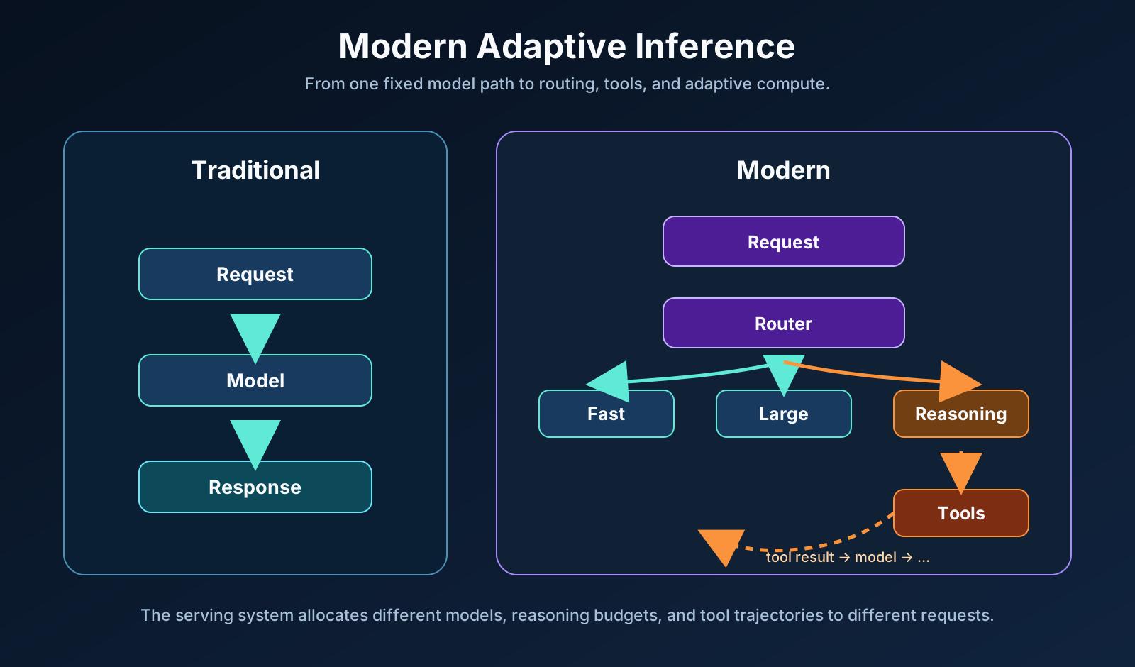
The next frontier is not simply a larger fixed model. It is inference-time scaling: choosing how much compute, memory, tool use, and verification a particular request deserves. Future systems will combine sparse capacity, cache-aware long context, adaptive reasoning budgets, speculative execution, and trajectory-level schedulers. The engineering challenge is to make that adaptation predictable, observable, and economically viable at production scale.
8. Comparing modern models
The table below is a mental map of the industry’s design space rather than a benchmark leaderboard. It separates the model’s architectural choice from the serving constraint that choice creates.
| Model | Architecture / strategy | Primary inference challenge | Key optimization | What it teaches |
|---|---|---|---|---|
| DeepSeek-V3 | MoE + MLA | Expert routing and KV memory | Sparse activation plus compressed KV state | Model architecture can directly reduce inference cost. |
| DeepSeek-R1 | Reasoning model | Increasing inference-time compute | Reasoning-time scaling | Compute can improve quality when allocated to the right requests. |
| DeepSeek-V4 | Trillion-scale MoE | Long context and distributed execution | Sparse activation plus efficient attention | Total parameters do not equal active computation. |
| Qwen3 | Thinking / non-thinking modes | Variable reasoning demand | Controllable thinking budget | Compute should adapt to task difficulty. |
| Qwen3.5 | Dense/MoE models plus agentic workflows | Multi-step inference trajectories | Adaptive model and compute selection | Agentic workloads change serving economics. |
| Qwen3.5-Omni | Hybrid Attention MoE | Multimodal, long-sequence serving | Efficient hybrid attention | Multimodal inference introduces new bottlenecks. |
| Kimi K2 | Trillion-scale MoE | Expert routing | Sparse activation | Trillion-scale models can be practical when active work is bounded. |
| Kimi K2.6 | Agentic MoE | Long-horizon execution | Agent-oriented inference | The number of model calls can matter more than a small per-token speedup. |
| Kimi K3 | 2.8T parameters with 1M context | Massive memory demand and context management | KDA and related architectural changes | Context length becomes a systems problem. |
| GPT-5 | Routed unified system | Choosing an inference path | Real-time routing | Model selection is itself an optimization. |
| Future reasoning models | Adaptive inference | Compute allocation | Inference-time scaling | Inference becomes dynamic. |
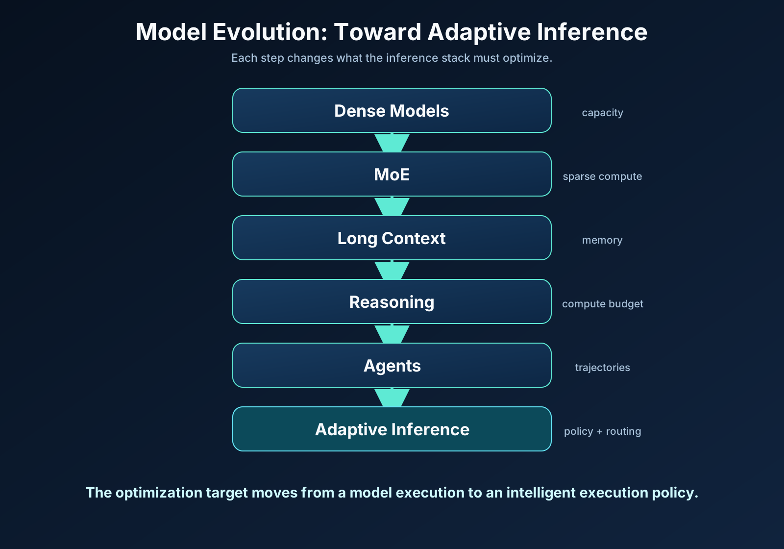
The common direction is adaptive computation: do not run the most expensive path for every token, request, or context. Choose a path that matches the difficulty, modality, context, and latency/cost budget.
9. Current trends in inference
- Lower precision is becoming a system feature. FP8, INT8, INT4, and newer low-precision paths reduce capacity and bandwidth, but need hardware-aware kernels and accuracy validation.
- KV cache is a strategic resource. Long contexts, shared prefixes, and high concurrency make cache allocation and reuse central to service economics.
- Sparse models shift the bottleneck to communication. MoE trades dense arithmetic for routing and all-to-all traffic.
- Prefill and decode are being optimized separately. Their resource profiles and SLOs are different enough to justify separate scheduling or hardware pools.
- Inference is moving from model serving to trajectory serving. Agents turn one user request into a graph of model calls, tools, and context updates.
- Tail latency is receiving more attention. Average tokens/s hides queues, stragglers, cache misses, and cross-node contention that users experience directly.
10. What the future inference stack looks like
The future stack is likely adaptive across layers:
request
  ↓
policy/router ── chooses model, reasoning budget, cache policy, and priority
  ↓
prefill pool / decode pool ── independently scheduled and capacity-managed
  ↓
runtime ── continuous batching, paged KV, prefix sharing, communication overlap
  ↓
compiler and kernels ── precision-, shape-, and hardware-aware execution
  ↓
GPU cluster and network ── HBM capacity/bandwidth plus topology-aware collectives
This stack requires co-design. An MoE model benefits from grouped-GEMM kernels, an expert-aware runtime, and a high-bandwidth network. A long-context model benefits from cache-efficient attention, paging, and memory-aware scheduling. An adaptive reasoning product benefits from a reliable router and metrics that measure quality, spend, and latency together.
A practical operating loop remains essential:
- Define SLOs and cost targets.
- Profile request queues, TTFT/TPOT, cache behavior, GPU timelines, and network traffic.
- Identify the current bottleneck.
- Apply the optimization that targets that bottleneck.
- Re-measure, because the bottleneck has probably moved.
11. Conclusion
Modern LLM inference is not “load the model and run it.” It is a coordinated system of routing, prefill, decode, KV-cache management, batching, compilation, kernels, accelerators, and networking.
The key principles are:
- Treat prefill and decode as distinct workloads.
- Size systems for weights and KV cache, not parameters alone.
- Use quantization, fusion, attention improvements, batching, and parallelism to address specific measured constraints.
- Expect sparse models to trade compute for communication complexity.
- Optimize end-to-end trajectories as models become reasoning- and agent-oriented.
The next generation of inference engineering will be defined by adaptive execution: selecting the right model path, precision, cache strategy, hardware placement, and reasoning budget for each request. The winning stack will not simply execute more FLOPS—it will deliver the right amount of intelligence at the right latency and cost.